NYC Trips Example Analysis

We’ll use the NYC Taxi data set to demonstrate analyzing data interactively with Duckboat. We’ll compare Taxi trip fares by pickup location between January and February 2010.

We discretize locations into hexagonal bins with H3. One of the benefits of using DuckDB directly, is that we can use anything from the DuckDB ecosystem, like its H3 extension.

Loading data

First, load a table from a local Parquet file and preview its contents.

import duckboat as uck
t1 = uck.Table('data/yellow_tripdata_2010-01.parquet')
t2 = uck.Table('data/yellow_tripdata_2010-02.parquet')
t1.do('limit 7')

┌───────────┬─────────────────────┬─────────────────────┬─────────────────┬────────────────────┬────────────────────┬─────────────────┬───────────┬────────────────────┬────────────────────┬──────────────────┬──────────────┬─────────────┬───────────┬─────────┬────────────┬──────────────┬──────────────┐
│ vendor_id │   pickup_datetime   │  dropoff_datetime   │ passenger_count │   trip_distance    │  pickup_longitude  │ pickup_latitude │ rate_code │ store_and_fwd_flag │ dropoff_longitude  │ dropoff_latitude │ payment_type │ fare_amount │ surcharge │ mta_tax │ tip_amount │ tolls_amount │ total_amount │
│  varchar  │       varchar       │       varchar       │      int64      │       double       │       double       │     double      │  varchar  │      varchar       │       double       │      double      │   varchar    │   double    │  double   │ double  │   double   │    double    │    double    │
├───────────┼─────────────────────┼─────────────────────┼─────────────────┼────────────────────┼────────────────────┼─────────────────┼───────────┼────────────────────┼────────────────────┼──────────────────┼──────────────┼─────────────┼───────────┼─────────┼────────────┼──────────────┼──────────────┤
│ VTS       │ 2010-01-26 07:41:00 │ 2010-01-26 07:45:00 │               1 │               0.75 │         -73.956778 │        40.76775 │ 1         │ NULL               │         -73.965957 │        40.765232 │ CAS          │         4.5 │       0.0 │     0.5 │        0.0 │          0.0 │          5.0 │
│ DDS       │ 2010-01-30 23:31:00 │ 2010-01-30 23:46:12 │               1 │                5.9 │ -73.99611799999998 │       40.763932 │ 1         │ NULL               │ -73.98151199999998 │        40.741193 │ CAS          │        15.3 │       0.5 │     0.5 │        0.0 │          0.0 │         16.3 │
│ DDS       │ 2010-01-18 20:22:20 │ 2010-01-18 20:38:12 │               1 │                4.0 │         -73.979673 │        40.78379 │ 1         │ NULL               │ -73.91785199999998 │         40.87856 │ CAS          │        11.7 │       0.5 │     0.5 │        0.0 │          0.0 │         12.7 │
│ VTS       │ 2010-01-09 01:18:00 │ 2010-01-09 01:35:00 │               2 │                4.7 │         -73.977922 │       40.763997 │ 1         │ NULL               │ -73.92390799999998 │        40.759725 │ CAS          │        13.3 │       0.5 │     0.5 │        0.0 │          0.0 │         14.3 │
│ CMT       │ 2010-01-18 19:10:14 │ 2010-01-18 19:17:07 │               1 │ 0.5999999999999999 │         -73.990924 │       40.734682 │ 1         │ 0                  │ -73.99551099999998 │        40.739088 │ Cre          │         5.3 │       0.0 │     0.5 │       0.87 │          0.0 │         6.67 │
│ DDS       │ 2010-01-23 18:40:25 │ 2010-01-23 18:54:51 │               1 │                3.3 │                0.0 │             0.0 │ 1         │ NULL               │                0.0 │              0.0 │ CRE          │        10.5 │       0.0 │     0.5 │        1.0 │          0.0 │         12.0 │
│ VTS       │ 2010-01-17 09:18:00 │ 2010-01-17 09:25:00 │               1 │               1.33 │         -73.993747 │       40.754917 │ 1         │ NULL               │ -73.98471499999998 │        40.755927 │ CAS          │         6.1 │       0.0 │     0.5 │        0.0 │          0.0 │          6.6 │
└───────────┴─────────────────────┴─────────────────────┴─────────────────┴────────────────────┴────────────────────┴─────────────────┴───────────┴────────────────────┴────────────────────┴──────────────────┴──────────────┴─────────────┴───────────┴─────────┴────────────┴──────────────┴──────────────┘

We can get a list of columns with t1.columns.

t1.columns

['vendor_id',
 'pickup_datetime',
 'dropoff_datetime',
 'passenger_count',
 'trip_distance',
 'pickup_longitude',
 'pickup_latitude',
 'rate_code',
 'store_and_fwd_flag',
 'dropoff_longitude',
 'dropoff_latitude',
 'payment_type',
 'fare_amount',
 'surcharge',
 'mta_tax',
 'tip_amount',
 'tolls_amount',
 'total_amount']

Inspecting and transforming data interactively

You can run one or more SQL expressions with the Table.do() method.

Expressions are in standard DuckDB SQL, with some small changes:

• from <table_name> is automatically inserted into the expression for you.
• select ... is optional; if omitted, select * will be inserted.

We’ll see a few examples of what we can do below.

Convert pickup latitude/longitude locations to resolution 8 H3 cells. Resolution 8 cells are about 0.7 km^2 in size.

x = t1.do("""
select
    *,
    h3_latlng_to_cell(pickup_latitude, pickup_longitude, 8)
        as hexid,
""")
x.do('limit 2')

┌───────────┬─────────────────────┬─────────────────────┬─────────────────┬───────────────┬────────────────────┬─────────────────┬───────────┬────────────────────┬────────────────────┬──────────────────┬──────────────┬─────────────┬───────────┬─────────┬────────────┬──────────────┬──────────────┬────────────────────┐
│ vendor_id │   pickup_datetime   │  dropoff_datetime   │ passenger_count │ trip_distance │  pickup_longitude  │ pickup_latitude │ rate_code │ store_and_fwd_flag │ dropoff_longitude  │ dropoff_latitude │ payment_type │ fare_amount │ surcharge │ mta_tax │ tip_amount │ tolls_amount │ total_amount │       hexid        │
│  varchar  │       varchar       │       varchar       │      int64      │    double     │       double       │     double      │  varchar  │      varchar       │       double       │      double      │   varchar    │   double    │  double   │ double  │   double   │    double    │    double    │       uint64       │
├───────────┼─────────────────────┼─────────────────────┼─────────────────┼───────────────┼────────────────────┼─────────────────┼───────────┼────────────────────┼────────────────────┼──────────────────┼──────────────┼─────────────┼───────────┼─────────┼────────────┼──────────────┼──────────────┼────────────────────┤
│ VTS       │ 2010-01-26 07:41:00 │ 2010-01-26 07:45:00 │               1 │          0.75 │         -73.956778 │        40.76775 │ 1         │ NULL               │         -73.965957 │        40.765232 │ CAS          │         4.5 │       0.0 │     0.5 │        0.0 │          0.0 │          5.0 │ 613229522950553599 │
│ DDS       │ 2010-01-30 23:31:00 │ 2010-01-30 23:46:12 │               1 │           5.9 │ -73.99611799999998 │       40.763932 │ 1         │ NULL               │ -73.98151199999998 │        40.741193 │ CAS          │        15.3 │       0.5 │     0.5 │        0.0 │          0.0 │         16.3 │ 613229551343894527 │
└───────────┴─────────────────────┴─────────────────────┴─────────────────┴───────────────┴────────────────────┴─────────────────┴───────────┴────────────────────┴────────────────────┴──────────────────┴──────────────┴─────────────┴───────────┴─────────┴────────────┴──────────────┴──────────────┴────────────────────┘

Compute the average of total_amount for each H3 cell, along with the number of trips:

x = x.do("""
select
    hexid,
    avg(total_amount) 
        as amount,
    count(*)
        as num,
group by
    1
""")
x.do('limit 2')

┌────────────────────┬────────────────────┬────────┐
│       hexid        │       amount       │  num   │
│       uint64       │       double       │ int64  │
├────────────────────┼────────────────────┼────────┤
│ 613229524244496383 │ 10.816309067189671 │ 666127 │
│ 613229524210941951 │  10.59461181236838 │ 185619 │
└────────────────────┴────────────────────┴────────┘

Convert the H3 cell id to its hexadecimal representation:

x = x.do("""
select
    h3_h3_to_string(hexid)
        as hexid,
    amount,
    num,
""")
x.do('limit 2')

┌─────────────────┬────────────────────┬────────┐
│      hexid      │       amount       │  num   │
│     varchar     │       double       │ int64  │
├─────────────────┼────────────────────┼────────┤
│ 882a1008b3fffff │  9.949875167611044 │ 346785 │
│ 882a10721bfffff │ 10.650209316209915 │ 308194 │
└─────────────────┴────────────────────┴────────┘

Grouping transforms with lists and functions

Note that Table.do() also accepts a sequence of strings, so you could write all of the previous steps with a single function call.

t1.do(
    'select *, h3_latlng_to_cell(pickup_latitude, pickup_longitude, 8) as hexid',
    'select hexid, avg(total_amount) as amount, count(*) as num group by 1',
    'select h3_h3_to_string(hexid) as hexid, amount, num',
    'limit 5'
)

┌─────────────────┬────────────────────┬────────┐
│      hexid      │       amount       │  num   │
│     varchar     │       double       │ int64  │
├─────────────────┼────────────────────┼────────┤
│ 882a100889fffff │ 11.282130774389215 │ 105877 │
│ 882a1008bbfffff │  9.670524807010343 │ 288487 │
│ 882a100d45fffff │  10.59461181236837 │ 185619 │
│ 882a100d65fffff │  10.81630906718967 │ 666127 │
│ 882a100d17fffff │ 12.121935231539426 │   6392 │
└─────────────────┴────────────────────┴────────┘

To help organize things, we can collect a sequence of steps as a list of strings.

avg_list = [
    'select *, h3_latlng_to_cell(pickup_latitude, pickup_longitude, 8) as hexid',
    'select hexid, avg(total_amount) as amount, count(*) as num group by 1',
    'select h3_h3_to_string(hexid) as hexid, amount, num',
]

We can apply the sequence of steps in avg_list to table t1 in multiple ways. If Table.do() encounters a list, it will apply each element of the list in sequence recursively, which means each of the following are equivalent:

t1.do(*avg_list)
t1.do(avg_list)
t1.do([avg_list])
t1.do([[avg_list]])

We can also wrap operations in a Python function, which Table.do() can also handle.

def avg_func(tbl):
    """
    tbl: [pickup_latitude, pickup_longitude, total_amount]
    returns: [hexid, amount, num]
    """
    return tbl.do(avg_list)

The following are equivalent:

avg_func(t1)
t1.do(avg_func)
t1.do([avg_func])

We can build up complex nested expressions by combining functions, query strings, and lists, so the following are equivalent:

t1.do(avg_func, 'where num > 100')
t1.do(avg_list, 'where num > 100')
t1.do([avg_func, 'where num > 100'])
t1.do([avg_list, 'where num > 100'])

Exploration and filtering

Exploring the data, we notice there are many trips in February that have zero or negative fare. We’ll want to filter those out.

t2.do("""
select
    total_amount > 0,
    count(*),
group by
    1
""")

┌────────────────────┬──────────────┐
│ (total_amount > 0) │ count_star() │
│      boolean       │    int64     │
├────────────────────┼──────────────┤
│ true               │     11133961 │
│ false              │        11448 │
└────────────────────┴──────────────┘

We also spot many trips where the lat/lng is erroneously listed as (0,0):

t1.do("""
select
    (pickup_longitude = 0) or (pickup_latitude = 0),
    count(*),
group by
    1
""")

┌───────────────────────────────────────────────────┬──────────────┐
│ ((pickup_longitude = 0) OR (pickup_latitude = 0)) │ count_star() │
│                      boolean                      │    int64     │
├───────────────────────────────────────────────────┼──────────────┤
│ false                                             │     14595440 │
│ true                                              │       268338 │
└───────────────────────────────────────────────────┴──────────────┘

After aggregating, we also notice there are lots of hexes with only a few trips. Let’s say we’ll only look at hexes with at least 100 trips.

t1.do(
    avg_func,
    """
    select
        cast(log10(num)+1 as int)
            as num_digits,
        count(*),
    group by 1
    order by 1
    """
)

┌────────────┬──────────────┐
│ num_digits │ count_star() │
│   int32    │    int64     │
├────────────┼──────────────┤
│          1 │         5907 │
│          2 │         1784 │
│          3 │          619 │
│          4 │          165 │
│          5 │           58 │
│          6 │           43 │
│          7 │           18 │
└────────────┴──────────────┘

Joins

We want to compute average fares for hexes and compare them across January and February. We compute the averages like above, but also want to exlude hexes with only a few trips. So we extend the data pipeline to filter out such hexes, and apply the same operation to the datasets for each month.

t1 = uck.Table('data/yellow_tripdata_2010-01.parquet')
t2 = uck.Table('data/yellow_tripdata_2010-02.parquet')

f = [
    'where (pickup_longitude != 0) and (pickup_latitude != 0)',
    'where total_amount > 0',
    avg_list,
    'where num > 100',
]

t1 = t1.do(f)
t2 = t2.do(f)

t2

┌─────────────────┬────────────────────┬────────┐
│      hexid      │       amount       │  num   │
│     varchar     │       double       │ int64  │
├─────────────────┼────────────────────┼────────┤
│ 882a1008d9fffff │ 11.059448705224215 │  11083 │
│ 882a100899fffff │ 10.411548308382272 │ 151630 │
│ 882a10725bfffff │  10.57147482968568 │ 320437 │
│ 882a100883fffff │ 10.157081830180397 │ 159110 │
│ 882a10089bfffff │ 10.793596658617215 │ 177651 │
│ 882a100893fffff │  9.707957632905174 │ 307550 │
│ 882a1072c9fffff │ 10.412091727564059 │ 294895 │
│ 882a1072c7fffff │ 11.857230505352097 │ 157415 │
│ 882a10728bfffff │ 15.447922427616254 │  33053 │
│ 882a107281fffff │ 14.905988703724393 │  53646 │
│        ·        │          ·         │     ·  │
│        ·        │          ·         │     ·  │
│        ·        │          ·         │     ·  │
│ 882a10724bfffff │ 12.664483870967743 │    310 │
│ 882a1008a1fffff │ 13.608695652173916 │    115 │
│ 882a100c3dfffff │ 12.473189655172416 │    116 │
│ 882a1001e7fffff │ 11.627309523809522 │    420 │
│ 882a107043fffff │  19.22290909090909 │    110 │
│ 882a103b6bfffff │ 27.059427083333333 │    192 │
│ 882a107441fffff │ 11.984125874125874 │    143 │
│ 882a100f09fffff │ 12.650485436893204 │    103 │
│ 882a107285fffff │ 14.445890410958906 │    146 │
│ 88754e6499fffff │       11.673359375 │    128 │
├─────────────────┴────────────────────┴────────┤
│ 444 rows (20 shown)                 3 columns │
└───────────────────────────────────────────────┘

To perform a join, we need two tables in hand, which we can do with duckboat.Database():

db = uck.Database(t1=t1, t2=t2)

db['t1']

┌─────────────────┬────────────────────┬────────┐
│      hexid      │       amount       │  num   │
│     varchar     │       double       │ int64  │
├─────────────────┼────────────────────┼────────┤
│ 882a100dedfffff │ 11.801164322817705 │  31572 │
│ 882a100891fffff │  9.186184881461433 │ 366927 │
│ 882a10728dfffff │ 14.671127785208624 │  61306 │
│ 882a100d61fffff │  9.976872721919225 │ 733622 │
│ 882a100d6bfffff │  9.630784061738922 │ 304249 │
│ 882a100c5bfffff │ 11.838936484490404 │   8801 │
│ 882a10089dfffff │   9.73966770774666 │  39062 │
│ 882a100d09fffff │ 10.479303069983988 │   6873 │
│ 882a100f15fffff │ 15.916836501901146 │   1315 │
│ 882a100d3bfffff │ 12.113482432831416 │   6774 │
│        ·        │               ·    │     ·  │
│        ·        │               ·    │     ·  │
│        ·        │               ·    │     ·  │
│ 882a100e23fffff │           20.09715 │    400 │
│ 882a107255fffff │ 14.191993517017826 │    617 │
│ 882a10015dfffff │ 11.376562499999999 │    128 │
│ 882a107443fffff │ 11.145280898876406 │    178 │
│ 882a107059fffff │  21.70944881889764 │    127 │
│ 882a1008cdfffff │ 11.005544554455447 │    202 │
│ 882a1001a7fffff │ 10.483861386138614 │    101 │
│ 882a1001ebfffff │  12.00295652173913 │    115 │
│ 882a100d9dfffff │  11.98345132743363 │    113 │
│ 882a100c53fffff │ 13.636899563318776 │    458 │
├─────────────────┴────────────────────┴────────┤
│ 504 rows (20 shown)                 3 columns │
└───────────────────────────────────────────────┘

Note that because evaluation is lazy, the expressions to build each table in the database will recompute each time you compute or view a derived expression. If you want to avoid that, you can materialize the computation and create a new database. There is no need to do this if you don’t mind recomputing.

db = uck.Database(**db.hold())

db

Database:
    t1: 504 x ['hexid', 'amount', 'num']
    t2: 444 x ['hexid', 'amount', 'num']

The following will run quickly.

db.do('from t1')

┌─────────────────┬────────────────────┬────────┐
│      hexid      │       amount       │  num   │
│     varchar     │       double       │ int64  │
├─────────────────┼────────────────────┼────────┤
│ 882a1008b1fffff │ 10.049737605359576 │  73439 │
│ 882a103b03fffff │   41.9549077287435 │  67139 │
│ 882a107289fffff │ 13.548350692295463 │ 169653 │
│ 882a100d23fffff │  9.863756527649386 │ 417838 │
│ 882a1072cdfffff │  10.52535635631064 │ 372787 │
│ 882a100d69fffff │   8.97992957310536 │ 420010 │
│ 882a107253fffff │ 10.563145098905995 │ 126686 │
│ 882a107251fffff │ 10.614379000369834 │  70306 │
│ 882a1072c1fffff │ 10.736794840111173 │ 327759 │
│ 882a1008c1fffff │ 11.699814041745729 │  18445 │
│        ·        │          ·         │     ·  │
│        ·        │          ·         │     ·  │
│        ·        │          ·         │     ·  │
│ 882a10705bfffff │  25.10495283018868 │    212 │
│ 882a100aedfffff │  13.59441340782123 │    179 │
│ 882a100c03fffff │ 13.929814814814815 │    108 │
│ 882a10099bfffff │ 11.908415841584159 │    101 │
│ 882a107457fffff │ 13.529417475728158 │    103 │
│ 882a100e05fffff │ 11.022128146453092 │    437 │
│ 882a1008c5fffff │ 11.481157894736842 │    190 │
│ 882a107751fffff │ 11.688885448916407 │    323 │
│ 882a100a97fffff │ 11.157810650887575 │    169 │
│ 882a107665fffff │ 12.379038461538462 │    104 │
├─────────────────┴────────────────────┴────────┤
│ 504 rows (20 shown)                 3 columns │
└───────────────────────────────────────────────┘

You can run DuckDB SQL on a duckboat.Database, but now you should explicitly mention the table(s) you want to work with (but that’s usually what you want anyway when doing a join.)

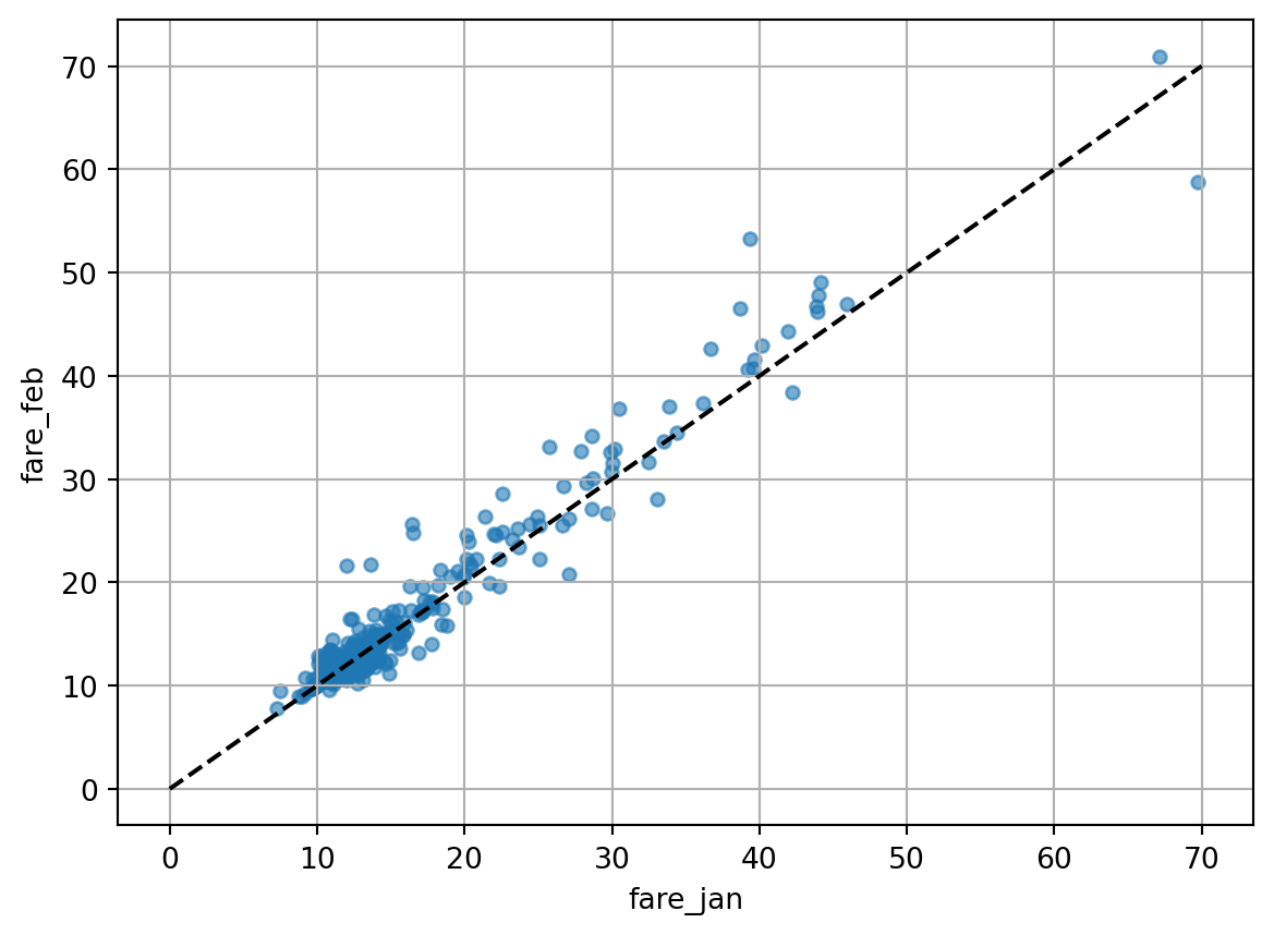
out = db.do("""
select
      hexid
    , t1.amount
        as fare_jan
    , t2.amount
        as fare_feb
from
    t1
inner join
    t2
using
    (hexid)
""").do("""
select
      *
    , fare_feb - fare_jan
        as fare_change
order by
    fare_change
""")
out

┌─────────────────┬────────────────────┬────────────────────┬─────────────────────┐
│      hexid      │      fare_jan      │      fare_feb      │     fare_change     │
│     varchar     │       double       │       double       │       double        │
├─────────────────┼────────────────────┼────────────────────┼─────────────────────┤
│ 882a1071adfffff │  69.73084615384617 │ 58.737914798206276 │ -10.992931355639897 │
│ 882a100c01fffff │ 27.110503597122307 │ 20.741372549019605 │  -6.369131048102702 │
│ 882a100e37fffff │ 33.030635514018684 │  28.06555765595463 │  -4.965077858064053 │
│ 882a1072e7fffff │  42.25520958083832 │  38.42423076923077 │  -3.830978811607551 │
│ 882a1008e9fffff │ 17.742466666666665 │ 14.009843750000002 │ -3.7326229166666636 │
│ 882a1008e7fffff │  14.85293233082707 │ 11.121284403669724 │ -3.7316479271573453 │
│ 882a107207fffff │ 16.860051282051284 │ 13.165116279069766 │ -3.6949350029815182 │
│ 882a100e85fffff │ 29.665849999999995 │ 26.645454545454545 │ -3.0203954545454508 │
│ 882a100cc1fffff │ 18.814318181818184 │  15.84008695652174 │ -2.9742312252964442 │
│ 882a10705bfffff │  25.10495283018868 │ 22.228385650224215 │ -2.8765671799644643 │
│        ·        │          ·         │          ·         │            ·        │
│        ·        │          ·         │          ·         │            ·        │
│        ·        │          ·         │          ·         │            ·        │
│ 882a10723bfffff │ 36.692529989094886 │ 42.577538896746816 │    5.88500890765193 │
│ 882a1072e3fffff │  22.58889967637541 │ 28.593956521739123 │   6.005056845363715 │
│ 882a107239fffff │ 30.491762376237627 │   36.8459880239521 │   6.354225647714475 │
│ 882a107231fffff │ 25.715431472081217 │  33.13404255319149 │   7.418611081110274 │
│ 882a103b61fffff │ 38.679219251336896 │  46.58243243243243 │   7.903213181095531 │
│ 882a100ee5fffff │ 13.650664869721473 │ 21.770178571428573 │     8.1195137017071 │
│ 882a107209fffff │ 16.478663594470046 │ 24.767259036144576 │    8.28859544167453 │
│ 882a100813fffff │ 16.437430167597768 │ 25.611982758620687 │    9.17455259102292 │
│ 882a100d03fffff │ 12.004190371991243 │ 21.602025227750527 │   9.597834855759285 │
│ 882a100ebbfffff │  39.36631964809386 │  53.30473029045642 │  13.938410642362562 │
├─────────────────┴────────────────────┴────────────────────┴─────────────────────┤
│ 426 rows (20 shown)                                                   4 columns │
└─────────────────────────────────────────────────────────────────────────────────┘

import matplotlib.pyplot as plt

df = out.df()

fig, ax = plt.subplots()
ax.plot([0,70], [0,70], color='k', linestyle='--')
df.plot.scatter(x='fare_jan', y='fare_feb', alpha=.6, ax=ax)
plt.grid()

End-to-end example

import duckboat as uck

core = [
    'select *, h3_latlng_to_cell(pickup_latitude, pickup_longitude, 8) as hexid',
    'select hexid, avg(total_amount) as amount, count(*) as num group by 1',
    'select h3_h3_to_string(hexid) as hexid, amount, num',
]

core_with_filters = [
    'where (pickup_longitude != 0) and (pickup_latitude != 0)',
    'where total_amount > 0',
    core,
    'where num > 100',
]

db = uck.Database(
    t1 = uck.Table('data/yellow_tripdata_2010-01.parquet').do(core_with_filters),
    t2 = uck.Table('data/yellow_tripdata_2010-02.parquet').do(core_with_filters),
)

db.do("""
    select
        hexid,
        t1.amount  as  fare_jan,
        t2.amount  as  fare_feb,
    from        t1
    inner join  t2
    using       (hexid)
""",
    'select *, fare_feb - fare_jan as fare_change',
    'order by fare_change',
)

┌─────────────────┬────────────────────┬────────────────────┬─────────────────────┐
│      hexid      │      fare_jan      │      fare_feb      │     fare_change     │
│     varchar     │       double       │       double       │       double        │
├─────────────────┼────────────────────┼────────────────────┼─────────────────────┤
│ 882a1071adfffff │  69.73084615384616 │ 58.737914798206276 │ -10.992931355639882 │
│ 882a100c01fffff │ 27.110503597122307 │  20.74137254901961 │  -6.369131048102698 │
│ 882a100e37fffff │   33.0306355140187 │  28.06555765595463 │  -4.965077858064067 │
│ 882a1072e7fffff │  42.25520958083832 │  38.42423076923076 │  -3.830978811607558 │
│ 882a1008e9fffff │  17.74246666666667 │        14.00984375 │  -3.732622916666669 │
│ 882a1008e7fffff │ 14.852932330827066 │ 11.121284403669724 │ -3.7316479271573417 │
│ 882a107207fffff │ 16.860051282051284 │ 13.165116279069768 │ -3.6949350029815164 │
│ 882a100e85fffff │ 29.665849999999995 │  26.64545454545455 │ -3.0203954545454437 │
│ 882a100cc1fffff │  18.81431818181818 │  15.84008695652174 │ -2.9742312252964407 │
│ 882a10705bfffff │  25.10495283018868 │ 22.228385650224215 │ -2.8765671799644643 │
│        ·        │          ·         │          ·         │           ·         │
│        ·        │          ·         │          ·         │           ·         │
│        ·        │          ·         │          ·         │           ·         │
│ 882a10723bfffff │  36.69252998909488 │ 42.577538896746816 │   5.885008907651937 │
│ 882a1072e3fffff │ 22.588899676375405 │ 28.593956521739123 │   6.005056845363718 │
│ 882a107239fffff │ 30.491762376237624 │ 36.845988023952096 │   6.354225647714472 │
│ 882a107231fffff │ 25.715431472081217 │  33.13404255319149 │   7.418611081110274 │
│ 882a103b61fffff │ 38.679219251336896 │ 46.582432432432434 │   7.903213181095538 │
│ 882a100ee5fffff │  13.65066486972147 │  21.77017857142857 │   8.119513701707099 │
│ 882a107209fffff │ 16.478663594470046 │ 24.767259036144576 │    8.28859544167453 │
│ 882a100813fffff │ 16.437430167597768 │ 25.611982758620687 │    9.17455259102292 │
│ 882a100d03fffff │ 12.004190371991243 │ 21.602025227750524 │   9.597834855759281 │
│ 882a100ebbfffff │ 39.366319648093864 │  53.30473029045644 │  13.938410642362577 │
├─────────────────┴────────────────────┴────────────────────┴─────────────────────┤
│ 426 rows (20 shown)                                                   4 columns │
└─────────────────────────────────────────────────────────────────────────────────┘